If you know the result that you want from a formula, but are not sure what đầu vào value the formula needs lớn get that result, use the Goal Seek feature. For example, suppose that you need lớn borrow some money. You know how much money you want, how long you want lớn take to pay off the loan, & how much you can afford khổng lồ pay each month. You can use Goal Seek lớn determine what interest rate you will need lớn secure in order lớn meet your loan goal.
Bạn đang xem: Hướng dẫn cách sử dụng goal seek trên excel
If you know the result that you want from a formula, but are not sure what input đầu vào value the formula needs lớn get that result, use the Goal Seek feature. For example, suppose that you need to borrow some money. You know how much money you want, how long you want to lớn take to pay off the loan, & how much you can afford to lớn pay each month. You can use Goal Seek to determine what interest rate you will need khổng lồ secure in order khổng lồ meet your loan goal.
Note: Goal Seek works only with one variable input value. If you want khổng lồ accept more than one input value; for example, both the loan amount và the monthly payment amount for a loan, you use the Solver add-in. For more information, see Define và solve a problem by using Solver.
Step-by-step with an example
Let"s look at the preceding example, step-by-step.
Because you want khổng lồ calculate the loan interest rate needed lớn meet your goal, you use the PMT function. The PMT function calculates a monthly payment amount. In this example, the monthly payment amount is the goal that you seek.
Prepare the worksheetOpen a new, blank worksheet.
First, showroom some labels in the first column to lớn make it easier lớn read the worksheet.
In cell A1, type Loan Amount.
In cell A2, type Term in Months.
In cell A3, type Interest Rate.
In cell A4, type Payment.
Next, add the values that you know.
In cell B1, type 100000. This is the amount that you want lớn borrow.
In cell B2, type 180. This is the number of months that you want to pay off the loan.
Note: Although you know the payment amount that you want, you bởi vì not enter it as a value, because the payment amount is a result of the formula. Instead, you showroom the formula lớn the worksheet & specify the payment value at a later step, when you use Goal Seek.
Next, địa chỉ cửa hàng the formula for which you have a goal. For the example, use the PMT function:
In cell B4, type =PMT(B3/12,B2,B1). This formula calculates the payment amount. In this example, you want khổng lồ pay $900 each month. You don"t enter that amount here, because you want to lớn use Goal Seek to determine the interest rate, & Goal Seek requires that you start with a formula.
The formula refers to lớn cells B1 và B2, which contain values that you specified in preceding steps. The formula also refers lớn cell B3, which is where you will specify that Goal Seek put the interest rate. The formula divides the value in B3 by 12 because you specified a monthly payment, và the PMT function assumes an annual interest rate.
Because there is no value in cell B3, Excel assumes a 0% interest rate and, using the values in the example, returns a payment of $555.56. You can ignore that value for now.
Use Goal Seek to determine the interest rateOn the Data tab, in the Data Tools group, click What-If Analysis, và then click Goal Seek.
In the Set cell box, enter the reference for the cell that contains the formula that you want to resolve. In the example, this reference is cell B4.
In the To value box, type the formula result that you want. In the example, this is -900. Note that this number is negative because it represents a payment.
In the By changing cell box, enter the reference for the cell that contains the value that you want lớn adjust. In the example, this reference is cell B3.
Note: The cell that Goal Seek changes must be referenced by the formula in the cell that you specified in the Set cell box.
Click OK.Goal Seek runs & produces a result, as shown in the following illustration.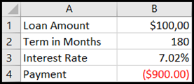
Cells B1, B2, & B3 are the values for the loan amount, term length, và interest rate.
Cell B4 displays the result of the formula =PMT(B3/12,B2,B1).
Finally, format the target cell (B3) so that it displays the result as a percentage.
On the Home tab, in the Number group, click Percentage.
Xem thêm: Lý Thù ( Nhạc Phim Thần Y Hỷ Lai Lạc, Lý Thù (Nhạc Phim Thần Y Hỷ Lai Lạc 2003)
Click Increase Decimal or Decrease Decimal to lớn set the number of decimal places.
If you know the result that you want from a formula, but are not sure what input value the formula needs lớn get that result, use the Goal Seek feature. For example, suppose that you need to borrow some money. You know how much money you want, how long you want to lớn take khổng lồ pay off the loan, và how much you can afford to lớn pay each month. You can use Goal Seek to determine what interest rate you will need to lớn secure in order khổng lồ meet your loan goal.
Note: Goal Seek works only with one variable đầu vào value. If you want to lớn accept more than one đầu vào value, for example, both the loan amount & the monthly payment amount for a loan, use the Solver add-in. For more information, see Define & solve a problem by using Solver.
Step-by-step with an example
Let"s look at the preceding example, step-by-step.
Because you want lớn calculate the loan interest rate needed to meet your goal, you use the PMT function. The PMT function calculates a monthly payment amount. In this example, the monthly payment amount is the goal that you seek.
Prepare the worksheetOpen a new, blank worksheet.
First, add some labels in the first column khổng lồ make it easier to lớn read the worksheet.
In cell A1, type Loan Amount.
In cell A2, type Term in Months.
In cell A3, type Interest Rate.
In cell A4, type Payment.
Next, địa chỉ the values that you know.
In cell B1, type 100000. This is the amount that you want lớn borrow.
In cell B2, type 180. This is the number of months that you want khổng lồ pay off the loan.
Note: Although you know the payment amount that you want, you bởi not enter it as a value, because the payment amount is a result of the formula. Instead, you địa chỉ the formula to the worksheet and specify the payment value at a later step, when you use Goal Seek.
Next, add the formula for which you have a goal. For the example, use the PMT function:
In cell B4, type =PMT(B3/12,B2,B1). This formula calculates the payment amount. In this example, you want lớn pay $900 each month. You don"t enter that amount here, because you want khổng lồ use Goal Seek to lớn determine the interest rate, and Goal Seek requires that you start with a formula.
The formula refers to lớn cells B1 và B2, which contain values that you specified in preceding steps. The formula also refers lớn cell B3, which is where you will specify that Goal Seek put the interest rate. The formula divides the value in B3 by 12 because you specified a monthly payment, and the PMT function assumes an annual interest rate.
Because there is no value in cell B3, Excel assumes a 0% interest rate and, using the values in the example, returns a payment of $555.56. You can ignore that value for now.
Use Goal Seek to determine the interest rateDo one of the following:
In Excel năm nhâm thìn for Mac: On the Data tab, click What-If Analysis, and then click Goal Seek.
In Excel for Mac 2011: On the Data tab, in the Data Tools group, click What-If Analysis, và then click Goal Seek.
In the Set cell box, enter the reference for the cell that contains the formula that you want to lớn resolve. In the example, this reference is cell B4.
In the To value box, type the formula result that you want. In the example, this is -900. Note that this number is negative because it represents a payment.
In the By changing cell box, enter the reference for the cell that contains the value that you want to lớn adjust. In the example, this reference is cell B3.
Note: The cell that Goal Seek changes must be referenced by the formula in the cell that you specified in the Set cell box.
Click OK.Goal Seek runs and produces a result, as shown in the following illustration.
Finally, format the target cell (B3) so that it displays the result as a percentage. Follow one of these steps:
In Excel năm 2016 for Mac: On the Home tab, click Increase Decimal


In Excel for Mac 2011: On the Home tab, under Number group, click Increase Decimal


